1. What do you mean by the term stochastic processes?
A stochastic process is a mathematical model used to describe systems or phenomena that evolve over time in a way that is inherently random. It involves a sequence of random variables, where each variable represents the state of the system at a given time. These processes are used to model the randomness and unpredictability in various real-world scenarios.
Key Characteristics:
- Randomness: The future state of the process is not entirely predictable and is described by a probability distribution.
- Time Indexing: The index set (often representing time) can be discrete (e.g., days, months) or continuous (e.g., every second, continuously).
- State Space: The set of possible values that the process can take.
2. What are the Types of Stochastic Processes?
Discrete-Time Stochastic Processes
- Definition: These processes are observed at specific, discrete points in time.
- Example: A simple random walk with Position changes by +1 or −1 each time step with some probability.
- Real-World Example: Imagine a game where you flip a coin every day. If it’s heads, you move one step forward; if it’s tails, you move one step backward. The position you are in after each coin flip is an example of a discrete-time stochastic process.
Continuous-Time Stochastic Processes
- Definition: These processes are observed continuously over time.
- Example: Brownian motion (Wiener process).
- Real-World Example: The random movement of pollen particles suspended in water, as observed under a microscope, is an example of Brownian motion. Similarly, the continuous fluctuation of stock prices in the market can be modeled as a continuous-time stochastic process.
3. What is Brownian motion?
In finance, Brownian motion, also known as a Wiener process, is a stochastic process that models the random, continuous movement of prices and other financial variables. It is characterized by stationary, independent increments and continuous paths. This process is essential for modeling the unpredictable behavior and volatility observed in financial markets, embodying the concept that small, random fluctuations in market factors can accumulate to significant effects over time. Brownian motion is fundamental to the theory of financial derivatives and risk management, providing a mathematical framework for modeling randomness that mirrors the erratic nature of markets.
Note: Standard Brownian Motion, also known as a Wiener process
The mathematical representation of Brownian motion, particularly in its most general form, is described through a stochastic differential equation (SDE). The equation for a standard Brownian motion, also known as a Wiener process, is given by: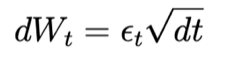 where:
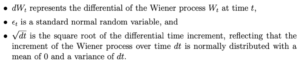 This simple form captures the essence of Brownian motion’s continuous and nowhere differentiable nature, with independent and stationary Gaussian increments.
4. What are the properties of Brownian Motion?
Brownian motion, or the Wiener process, has several key properties that make it fundamental in the modeling of stochastic processes in finance, physics, and mathematics. Here are the main properties:
- Continuous Paths: Brownian motion has continuous paths, meaning there are no jumps in the function; it is continuous everywhere. This property reflects the idea that, despite being unpredictable, the motion does not exhibit sudden leaps at any point in time.
- Stationary Increments: The increments of Brownian motion are stationary. This means that the statistical properties of any segment of the path depend only on the length of the segment, not on its location in time.
- Independent Increments: The increments of Brownian motion over non-overlapping intervals are independent of each other. This is a crucial property for modeling in finance as it implies that past movements of a stochastic variable (like a stock price) do not affect its future movements.
- Normally Distributed Increments: The increments of Brownian motion are normally distributed. For any time t and s, with t > s, the increment W(t) − W(s) is normally distributed with mean 0 and variance t − s.
- Origin: Brownian motion starts from zero, i.e., W(0) = 0.
- Martingale Property: Brownian motion has the martingale property with respect to the natural filtration it generates. This means the expected value of the future value conditioned on the past and present is equal to the present value, assuming a fair game in financial terms.
- Markov Property: Brownian motion is a Markov process. This means that the conditional probability distribution of future states of the process depends only on the present state, not on the sequence of events that preceded it.
These properties make Brownian motion a versatile tool in mathematical finance, particularly in the modeling of derivative pricing, risk management, and in the broader field of stochastic processes.
5. What is Geometric Brownian Motion (GBM)?
Geometric Brownian Motion (GBM) is a continuous-time stochastic process widely used in financial modeling, particularly for modeling the dynamics of stock prices and other financial assets. It is characterized by a logarithmic normal distribution of returns and captures both the deterministic and random aspects of asset price movements.
Mathematical Definition: The stochastic differential equation (SDE) that defines GBM is:![]() where:
where: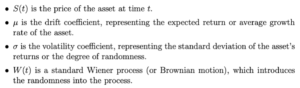
6. What are the key properties of GBM?
- Log-Normal Distribution: The asset price S(t) follows a log-normal distribution.
- The logarithm of the asset price, ln(S(t)), is normally distributed.
- The asset price S(t) is always positive, making it suitable for modeling stock prices.
- Drift and Volatility:
- Drift (μ): Represents the expected rate of return or average growth rate of the asset, introducing a deterministic trend in the price path.
- Volatility (σ): Represents the standard deviation of the asset’s returns, capturing randomness or uncertainty in price movements. It scales the random component of the process.
- Continuous Paths: GBM paths are continuous over time, meaning there are no jumps or discontinuities in the price process. This reflects the smooth evolution of asset prices.
- Independent Increments: The increments of the Wiener process W(t) are independent. Future price movements are independent of past movements, conditional on the current price.
- Markov Property: GBM has the Markov property:
- The future evolution of the process depends only on the current state.
- The price at any future time depends only on the current price, not the process’s history.
- Scaling Property: The increments of GBM over non-overlapping intervals are independent and identically distributed, ensuring the process is self-similar.
7. How does GBM differ from Arithmetic Brownian motion?
Geometric Brownian Motion (GBM) and Arithmetic Brownian Motion (ABM) are both stochastic processes used to model the evolution of variables over time. However, they have distinct characteristics and are used in different contexts. Here are the key differences between GBM and ABM:
Geometric Brownian Motion (GBM)
The stochastic differential equation (SDE) for GBM is:![]() Here, S(t) represents the process at time t, μ is the drift coefficient, σ is the volatility coefficient, and W(t) is a standard Wiener process.
Here, S(t) represents the process at time t, μ is the drift coefficient, σ is the volatility coefficient, and W(t) is a standard Wiener process.
Properties:
- Log-Normal Distribution: The logarithm of S(t) is normally distributed, making S(t) itself log-normally distributed.
- Non-Negative Values: Since S(t) is always positive, GBM is suitable for modeling asset prices and other quantities that cannot be negative.
- Proportional Changes: The relative change in S(t) is normally distributed. This means the process scales with the level of S(t).
Applications: Commonly used in financial modeling, especially for modeling stock prices and other financial assets in models like the Black-Scholes option pricing model.
Arithmetic Brownian Motion (ABM)
The stochastic differential equation (SDE) for ABM is:
![]() Properties:
Properties:
- Normal Distribution: The increments of X(t) are normally distributed, making X(t) itself normally distributed.
- Can Take Negative Values: X(t) can be negative, which may be unrealistic for modeling asset prices or quantities that must remain non-negative.
- Absolute Changes: The absolute change in X(t) is normally distributed, regardless of the current level of X(t).
Applications: Less commonly used for financial asset prices but can be used for modeling interest rates, exchange rates, and other quantities where negative values might be realistic or acceptable.
8. Can GBM be used to model asset prices with jumps or non-continuous features?
Geometric Brownian Motion (GBM) is not suitable for modeling asset prices with jumps or non-continuous features because it assumes continuous paths and normal distribution of returns. However, there are extensions and alternative models designed to handle jumps and discontinuities in asset prices. Here are some of the key models:
1. Jump-Diffusion Models
These models incorporate both continuous Brownian motion and discrete jumps. The most famous jump-diffusion model is the Merton model.
Merton’s Jump-Diffusion Model:
![]()
where:
- J(t) is a jump process, typically modeled as a Poisson process, which captures the jumps.
- dJ(t) represents the size and frequency of jumps.
2. Lévy Processes
Lévy processes generalize Brownian motion by allowing for jumps. They are used to model asset prices that exhibit discontinuities.
Example: Variance Gamma Process
- This process is used to capture the leptokurtic and skewed nature of asset returns.
- It combines Brownian motion with a Gamma process to introduce jumps and higher moments.
While GBM is a foundational model in finance, it assumes continuous paths and normally distributed returns, making it unsuitable for capturing jumps and other non-continuous features in asset prices. For more realistic modeling of such features, jump-diffusion models, Lévy processes, and stochastic volatility models with jumps are used. These models incorporate both continuous and discontinuous elements to better capture the behavior of financial assets in real markets.
9. Can you explain the concept of correlated processes in GBM?
In financial modeling, it is often necessary to model multiple assets whose prices may be correlated. When dealing with Geometric Brownian Motion (GBM) for multiple assets, the concept of correlated processes becomes important. Here’s an explanation of how correlated processes work in the context of GBM:
Correlated GBM Processes: When modeling the prices of multiple assets, we may assume that the Wiener processes (Brownian motions) driving these assets are correlated. This is because asset prices often move together due to common market factors or economic conditions.
Mathematical Representation: Consider two assets with prices S1(t) and S2(t) that follow GBM. Their stochastic differential equations (SDEs) are: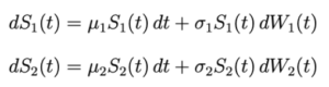 where:
![]() Correlation between Wiener Processes: To model the correlation between the two assets, we introduce a correlation coefficient ρ such that:
Correlation between Wiener Processes: To model the correlation between the two assets, we introduce a correlation coefficient ρ such that:
![]() This means that the increments of W1(t) and W2(t) are correlated with correlation coefficient ρ, where ρ ranges between -1 and 1.
This means that the increments of W1(t) and W2(t) are correlated with correlation coefficient ρ, where ρ ranges between -1 and 1.
- ρ = 1 means perfect positive correlation.
- ρ = −1 means perfect negative correlation.
- ρ = 0 means no correlation.
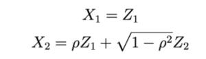
Constructing Correlated Wiener Processes: To simulate correlated Wiener processes, we can use the Cholesky decomposition or other techniques to generate correlated random variables. If Z1 and Z2 are two independent standard normal random variables, we can construct two correlated normal random variables X1 and X2 as follows:
10. How is Brownian motion applied in the modeling of financial markets?
In finance, Brownian motion is employed extensively to simulate the unpredictable behavior of financial instruments and market dynamics. Here’s how it is commonly used:
- Stock Price Modeling: Brownian motion underpins the geometric Brownian motion (GBM) model, which is prevalent in modeling stock prices. GBM assumes that the logarithmic returns of stock prices, not the prices themselves, are normally distributed and exhibit no memory of past movements, characterizing the unpredictable and independent nature of stock market movements.
- Option Pricing: Central to the Black-Scholes model for European option pricing, Brownian motion models the random trajectory of underlying asset prices. This model utilizes the properties of geometric Brownian motion, assuming constant drift (representative of average return) and volatility (standard deviation of returns), to derive an analytical formula for pricing options.
- Risk Management: Brownian motion assists in the computation of Value at Risk (VaR) and conducting stress tests in risk management frameworks. These tools are critical for understanding potential losses in investment portfolios under varying market conditions, based on simulations that project future price movements using Brownian motion.
- Interest Rate Modeling: In interest rate modeling, processes such as the Vasicek and Cox-Ingersoll-Ross models incorporate Brownian motion to depict the evolution of interest rates over time. This stochastic approach is vital for accurately pricing bonds and other interest-dependent securities.
- Foreign Exchange and Commodities: The pricing models for foreign exchange and commodities often use geometric Brownian motion to simulate price movements. This approach aids in derivative pricing and risk management by capturing the unpredictability of these markets.
- Brownian motion’s ability to represent the stochastic and independent nature of market variables makes it an indispensable tool in quantitative finance, supporting various pricing, trading, and risk management activities.
Interview Questions on Ito’s Lemma
1. What is Itô’s Lemma?
 2. What is the significance of the terms in Itô’s Lemma?
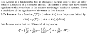 Significance of Each Term:
∂f/∂t dt:
- Significance: This term represents the direct change in the function f with respect to time, holding the stochastic process X(t) constant. It captures the explicit time dependence of f.
∂f/∂X · μ dt:
- Significance: This term captures the change in the function f due to the drift component μ of the stochastic process X(t). It represents the deterministic trend in X(t) and its impact on f.
1/2 · ∂²f/∂X² · σ² dt:
- Significance: This second-order term accounts for the curvature of the function f with respect to the stochastic variable X(t). It captures the impact of the variance of the stochastic process on f. The presence of ∂²f/∂X² indicates how the curvature of f influences its behavior under random fluctuations, while σ² scales this effect according to the volatility of X(t). This term is crucial for accurately modeling the effect of stochastic volatility and ensuring the correct application of Itô calculus.
∂f/∂X · σ dW(t):
- Significance: This term represents the change in f due to the stochastic component of the process X(t). It captures the instantaneous impact of the random fluctuations in X(t), scaled by the function’s sensitivity to X(t) (∂f/∂X) and the volatility (σ). This term is responsible for the stochastic nature of the differential df.
Combined Significance:
Drift Term (∂f/∂t dt + ∂f/∂X · μ dt):
- These terms together capture the deterministic part of the change in f due to both explicit time dependence and the drift of the process X(t). They represent how f changes on average over time due to non-random factors.
Diffusion Term (1/2 · ∂²f/∂X² · σ² dt):
- This term adjusts the deterministic changes for the effect of randomness in X(t). It ensures that the impact of volatility is correctly accounted for in the dynamics of f.
Stochastic Term (∂f/∂X · σ dW(t)):
- This term introduces the randomness into the differential of f, reflecting the instantaneous effects of the stochastic process.
Each term in Itô’s Lemma has a specific role in capturing different aspects of the changes in a function of a stochastic process. Together, they provide a comprehensive framework for understanding and modeling the behavior of systems influenced by both deterministic and stochastic factors.
3. What are some applications where Itô’s Lemma is applied?
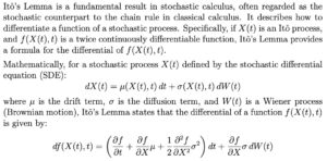
Itô’s Lemma is a fundamental tool in stochastic calculus with a wide range of applications, particularly in finance and other fields involving stochastic processes. Here are some key applications:
1. Derivative Pricing
Black-Scholes Model: Itô’s Lemma is used to derive the Black-Scholes partial differential equation, which forms the basis for the Black-Scholes option pricing model. This model provides a theoretical estimate of the price of European-style options.
2. Interest Rate Modeling
Models such as Vasicek and CIR: Itô’s Lemma is used to derive the dynamics of interest rates in models like the Vasicek and Cox-Ingersoll-Ross (CIR) models. These models are used to price interest rate derivatives and manage interest rate risk.
3. Stochastic Volatility Models
Models such as Heston Model and SABR Model: Itô’s Lemma is used to derive the dynamics of both the asset price and the stochastic volatility process. In these models, volatility is itself a stochastic process, and Itô’s Lemma helps in computing how functions of these processes evolve.
4. How is Itô’s Lemma used to derive the stochastic differential equation for geometric Brownian motion?
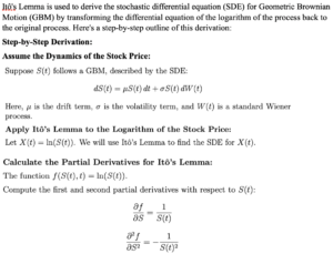
Itô’s Lemma is used to derive the stochastic differential equation (SDE) for Geometric Brownian Motion (GBM) by transforming the differential equation of the logarithm of the process back to the original process. Here’s a step-by-step outline of this derivation:
Step-by-Step Derivation:
Assume the Dynamics of the Stock Price:
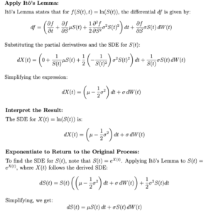 Summary:
By applying Itô’s Lemma to the logarithm of the stock price, we derive the SDE for the log of the stock price, which captures the drift and volatility of the process. We then exponentiate this result to obtain the original SDE for the stock price itself. This SDE characterizes the Geometric Brownian Motion, commonly used to model stock prices in financial mathematics.
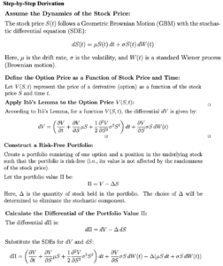
 5. How is Itô’s Lemma applied in deriving the Black-Scholes partial differential equation?
Itô’s Lemma plays a crucial role in deriving the Black-Scholes partial differential equation (PDE), which is fundamental in the pricing of options. Here’s a step-by-step outline of how Itô’s Lemma is applied in this derivation:
Step-by-Step Derivation
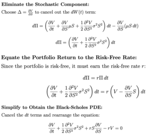 Conclusion:
Itô’s Lemma is crucial in transforming the stochastic differential equation of the stock price into a partial differential equation for the option price. This Black-Scholes PDE forms the foundation for pricing European options and other derivatives, allowing for the derivation of analytical solutions like the Black-Scholes formula for option pricing.
6. What are some limitations or challenges in applying Itô’s Lemma?
Itô’s Lemma is a powerful tool in stochastic calculus, but its application comes with several limitations and challenges:
1. Assumptions on Differentiability:
- Challenge: Itô’s Lemma requires the function f(X(t), t) to be twice continuously differentiable with respect to X(t) and continuously differentiable with respect to t.
- Limitation: In many practical applications, especially in finance, functions might not meet these smoothness conditions. For instance, payoff functions of some financial derivatives (like digital options) are not differentiable.
2. Complexity of Multiple Variables:
- Challenge: When dealing with multiple stochastic variables, applying Itô’s Lemma becomes significantly more complex.
- Limitation: Deriving the necessary partial derivatives and ensuring all terms are correctly accounted for can be mathematically intensive and prone to error.
3. Non-Standard Processes:
- Challenge: Itô’s Lemma applies specifically to Itô processes. Other types of stochastic processes, such as those involving jumps or those that follow a different type of noise (e.g., fractional Brownian motion), require different approaches or extensions of Itô’s Lemma.
- Limitation: The applicability of Itô’s Lemma is restricted to processes driven by standard Brownian motion, limiting its use in models incorporating discontinuities or more complex stochastic behaviors.
4. Numerical Implementation:
- Challenge: Implementing Itô’s Lemma in numerical simulations requires discretization of continuous processes.
- Limitation: Discretization can introduce approximation errors, and care must be taken to choose appropriate time steps and numerical methods to minimize these errors.
5. Real-World Data and Model Assumptions:
- Challenge: Real-world data often exhibit properties (e.g., heavy tails, volatility clustering) that standard models based on Itô’s Lemma (like Geometric Brownian Motion) do not capture well.
- Limitation: The simplifying assumptions necessary for applying Itô’s Lemma may not hold in practice, leading to models that can be inaccurate or misleading.
6. Handling Boundary Conditions:
- Challenge: When applying Itô’s Lemma to problems involving boundaries (e.g., in barrier options), handling the boundary conditions correctly is crucial.
- Limitation: Misapplying boundary conditions can lead to incorrect solutions, and the correct application can be mathematically intricate.
Summary: While Itô’s Lemma is a fundamental and versatile tool in stochastic calculus, its application is not without challenges. Issues related to differentiability, complexity in multiple variables, applicability to non-standard processes, numerical implementation, real-world data fit, interpretation in complex models, boundary conditions, and computational cost all need careful consideration to ensure accurate and meaningful results. Practitioners must be aware of these limitations and apply Itô’s Lemma judiciously within its valid context.